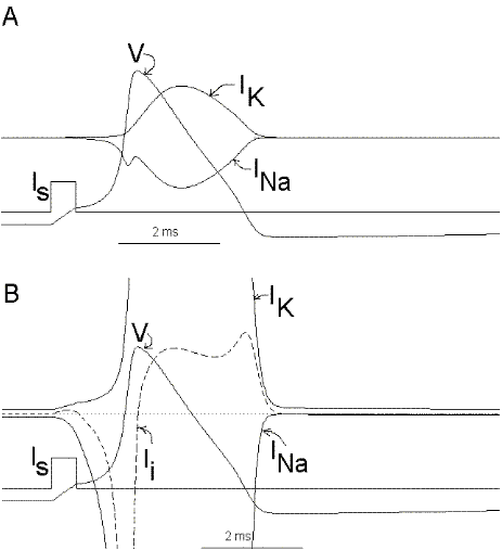
It is now possible to follow, step by step, the events leading to the potential rise and fall during an action potential. Suppose that we apply a small depolarizing current pulse to our axon with the axial wire (which also prevents propagation). Plate 3 shows a series of snapshots of the electrical equivalent circuit of the membrane including the voltage dependent Na and K channels. The branches are indicated with their reversal potentials and conductances: Na (for sodium), K (for potassium) and L (for leakage). The equilibrium potentials are indicated next to the corresponding batteries. The membrane potential is indicated in the bottom of the capacitor branch, and, as usual, the external side (top, in the figure) is referred as ground or zero potential. To the right bof each panel there is a plot of the membrane voltage (V) and the total ionic current (Ii). Concommitant with Plate 3 we must look at Fig 29. Fig. 29A shows a plot of the membrane action potential (V) as a result of the stimulating current pulse Is and the underlying Na and K currents through the membrane. Fig 29B is equivalent to Fig 29A, except that the currents are enlarged 20 times and the total ionic current (Ii=INa+IK+IL) is also shown.
In the resting condition, there is no current circulation between inside and outside which means that the sum of currents through all the four branches is equal to zero (Plate 3A and Fig. 29B). We also know that in this resting condition the value of gNa is much smaller than gK and gL, therefore most of the current will be across the K branch and the leakage branch. As the resting potential is more positive than EK, the current in the K branch will be outward and as it is more negative than the value of EL the current will be inward in the leakage branch. The direction of the currents are indicated by the arrows and their intensity by the darkness in Plate 3 (Membrane AP in circuit executes by clicking here).
Figure 29. Ionic currents during the impulse. In part Bthe currents are magnified 20 times with respect to part A.
To initiate the action potential, we apply a current pulse directed outward by making the inside more positive. This is shown in Plate 3 as a current generator connected between the outside and inside of the axon when the switch is closed. As we have described above, the first event will be the charging of the membrane capacitance that will occur as most of the current will initially go in the capacitive branch and subsequently through the Na, K and leakage branches in proportion to their conductances which will be preferentially through the K and leakage at short times (plate 3B). As the capacitance gets charged, the potential becomes more positive and gNa starts increasing (or RNa decreasing) which produces an inward current through the Na branch. Then the pulse of current is terminated and the total membrane current is again zero. However, there is outward K and leakage current, and inward Na current which keeps increasing until it becomes equal to the sum of IL and IK (Fig. 29B). The reason why the inward sodium current increases is because the membrane has been depolarized and the voltage-sensitive Na channels have been activated while K channels, which are slower to activate, have not responded yet to the depolarization. This is clearly seen in the trace of Ii shown Fig 29B, which crosses the zero line. At that time, if gNa is still increasing, inward Na current will predominate (see Fig 29B) and as more Na channels open, more inward current will flow which will depolarize the membrane even more, which will open more Na channels, etc (The Hodgkin cycle, Fig. 30). In this fashion, the membrane potential will tend to go to ENa, producing the upstroke of the action potential (Plate 3C). During this time, Na inactivation is increasing due to the depolarization. At the same time the K conductance, slower in turning on, starts increasing to the point that the total ionic current becomes outward through the K branch and the leakage branch, and eventually they cancel the Na current making the total ionic current equal zero (Plate 3D). After this, K outward current predominates and initiates the repolarization phase of the action potential (Plate 3E and Fig 29). Later, gK predominates pushing the potential towards the value of EK seen as the underswing of the action potential where gK is high but the current is low because V is too close to EK (see Plate 3F and Fig 29). After some time at this membrane potential, gK will again become small, producing a return of the membrane potential towards its normal resting value (as in Plate 3A).
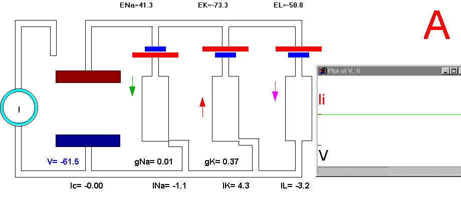
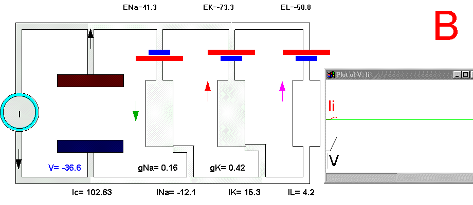
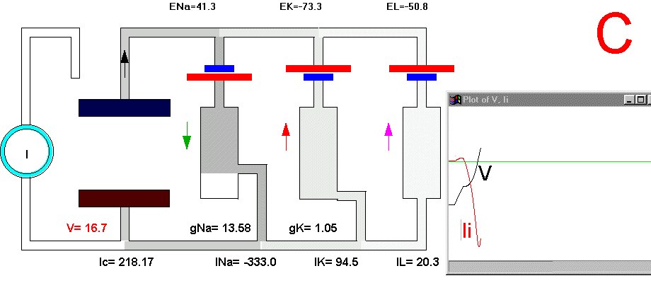
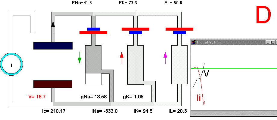
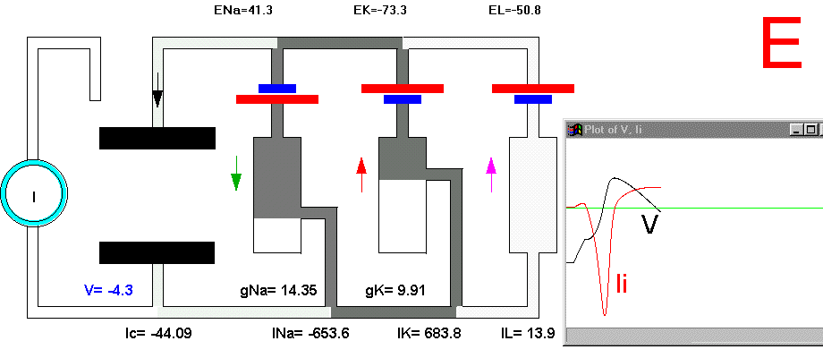
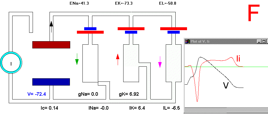
Plate 3. Currents and conductances in the equivalent circuit of the membrane during the action potential
There are some important points that must be explained in more detail in this sequence of events. In the resting state, there is no net current through the membrane but there is current circulation through the different branches (see, for example, Plate 3E). The applied pulse of current produces an outward (positive) current through the membrane that results in a depolarization of the membrane. If we neglect the current through gL and gNa, we find that the voltage across the membrane is the sum of EK plus the voltage drop across gK which has the opposite polarity. When the membrane potential has become depolarized enough such that gNa is increased, then the current through the Na branch becomes much larger and inward. As gNa increases, the voltage drop across gNa decreases ( V(across gNa)=INa/gNa ) and the internal potential tends to be closer to ENa, that is, positive inside. Notice that this is a case where an inward current is producing a depolarization, which is exactly the opposite that occurred during the early phase of depolarization, when the pulse of current was still present. If we look at the direction of the current in the capacitor branch of the membrane, however, we see that it is always an outward current during depolarization and an inward current during repolarization (Plate 3), as is expected because the voltage across the membrane is the voltage across the capacitor, which must be charged positively inside for depolarization, or negatively inside for hyperpolarization.
Our analysis of the generation of the action potential has been carried out in an axon with an axial wire. This was done to simplify the situation by preventing the propagation of the changes in membrane potential. In fact, with the axial wire, the voltage of the membrane along the whole stretch of axon changes simultaneously. Now we have to apply this knowledge to the real axon which does not have an axial wire in it. This means that we have to understand the consequences of the geometry of the axon on the current circulation across the membrane and along the axon. To proceed, we will first analyze the properties of a cylindrical axon when we apply very small current pulses. We will first use small pulses to prevent the initiation of the action potential, allowing us to understand the membrane potential changes and current circulation without the complications introduced by the voltage dependent conductances. After we have a clear idea of the current flow and membrane potential changes along the axon will we be in a position to extend the analysis for larger pulses that elicit changes of the Na and K conductances and from there follow the series of events that produce the propagation of the action potential.
The simple RC model of the membrane analyzed at the beginning of these notes is only valid provided there are no potential gradients in the inside or outside solutions. Here we are going to extend our analysis to include the geometry of the axon. It is important to realize that this analysis will be first done with a passive RC circuit, that is, with no voltage dependent conductances. Once we understand this simpler situation, we will incorporate the properties of the channels as we studied them before. Click here to execute an experiment on cable properties of the axon.
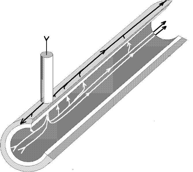
Figure 31. Longitudinal section of an axon showing a few lines of current flow near the electrode impaled at x=0. The other electrode is outside and far away.
Figure 31 shows a portion of an axon immersed in a conductive solution. There is an electrode penetrating the surface which is supplying current with respect to another electrode located outside, and the current circulation is pictured by a few lines of flow. If the membrane were a perfect insulator, no current would flow towards the external electrode. But due to the finite permeability of the axon, some current will circulate longitudinally in the axon interior, and exit through the surface membrane to be finally collected by the external electrode. It is clear then that due to the current circulation and the resistivity of the axoplasm, there will be voltage drops along the axon and none of the two sides of the membrane will be isopotential. Consequently we cannot use our simple membrane model to analyze the membrane potential along the axon.
The detailed analysis of this problem takes into account the geometry in three dimensions plus the time variable; the resulting equation is a partial differential equation in four independent variables. Considerable simplification can be achieved by assuming that all the lines of flow are
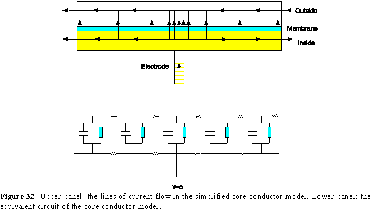
either parallel or perpendicular to the axon membrane and that there is no potential gradient radially inside or outside the axon (Fig. 32, upper panel). This seems like an arbitrary set of assumptions but it can be demonstrated that it is a good approximation for most of the practical cases. Under these conditions, our model gets reduced to a one-dimensional case with time as the second variable and it can be represented as a series of our membrane elements connected by internal and external resistances as shown in the lower panel of Fig. 32.
To proceed with the analysis, it will be necessary to define several parameters. Let us call ro the resistance of the outside solution per unit length, given in S/cm. This means that the total resistance on the outside for the segment of length Dx will be roDx. In the same manner we define ri as the internal resistance per unit length also in S/cm, giving the total internal resistance of the segment as ri Dx. Both the internal and external longitudinal currents will be given in A and the potentials in V. With regard to the currents perpendicular to the membrane we have to consider that the longer the segment the larger is the current, therefore we have to define them per unit length. We will then define the membrane current as im in A/cm. In this way the total membrane current will be imDx. The membrane resistance rm will be given in Scm, because as we take a longer piece of membrane the total resistance decreases.
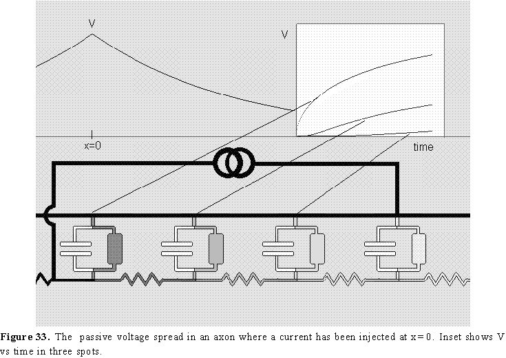
The analysis of the voltage distribution along the axon as a function of time for a stimulating current step in the center is shown schematically in Fig 33. In this case, the axon is immersed in a large bath of solution, therefore we may consider the external resistance close to zero, which makes the outside essentially isopotential. For this reason, the diagram is showing only the internal resistances connecting the membrane patches. Fig. 33 shows the current intensity as darkness in the wires, and it also shows the voltage distribution as a function of distance after we have waited a long time and all the capacitors have been charged to their final value (for this reason the currents are only in the resistive branches). When the pulse is suddenly applied, the current will go mainly to charge the membrane capacitance but most of this current will be taken by the capacitance closest to the electrode and much less by the capacitance further away because the internal resistance produces a voltage drop (V=ir) and less voltage will be seen by the distant capacitors. This initial capacitive charging may be considered like a short circuit at short times. As the capacitance near the electrode gets charged, the current in that region decreases and more can go to regions farther away and charge the rest of the axon capacitance. This means that regions far away from the current electrode will start increasing their voltage with a time lag. This is shown in the inset of Fig 33 where the time course of V has been plotted at three different points of the axon as indicated by the lines. It is obvious that none of these curves are exponentials as it was the case of the simple membrane model circuit. Even the time course of the voltage in the injection site is non-exponential. The actual function that relates V with x and t is complicated and includes error functions and will not be written here. Considerable simplification is achieved at long times when all the capacitors have been charged. In that case V(x), when t is large, is given by

for x>0 (replace x by -x for x<0).
I is the stimulating current and l is the space constant defined as

In the case of high external resistance ro, the definition of l includes the sum of ri + ro in the denominator. l represents the distance that one must travel from the injection site to record a voltage that is 0.37 (or 1/e) the value of the voltage at the injection site. As l increases, the spread of the voltage change also increases.
The value of l depends on the
membrane resistance and internal resistance. Our resistances have been expressed
pe unit length. We can compare the value of l
in different cells if we use specific quantities, that is, independent of geometry.
Thus rm=Rm/2Ba,
where Rm is the specific membrane resistance in Scm2
and a is the radius of the fiber. Also ri=Ri
/Ba2, where Ri
is the specific resistance of the axoplasm in Scm.
Replacing these expressions in the equation for 8,
we get

where we can see that the space constant is proportional to the square root
of the radius.
We are finally in a position to explain the propagation of the action potential. We know the details of the relation between membrane potential V and membrane current i at any point along the axon, therefore our task is to put together the relation of i and V at any point with the circulation of currents between different points along the axon.
The events during the action potential propagation (Fig. 34) are similar to the case of the space-clamped (axon with an axial wire) membrane described above, except that the stimulus is not external but is provided by another stretch of axon that has been excited. Suppose that we are considering eight small patches of membrane far from the stimulating electrode which, in turn, is located to the left in Fig. 34. Each panel of Fig. 34 has two parts: the top inset to the right represents the time course of the membrane potential in the three patches marked blue red and green with traces that are color-coded accordingly. The main region represents the membrane patches with each membrane patch with its capacitance (the long horizontal bars color coded according to the membrane potential), the four membrane current paths: capacitive, Na conductance (in green), the K conductance (in cyan) and the leak conductance (in white). The patches of membrane are interconnected beween them by the resistance of the external medium and the internal resistance of internal medium (axoplasm). The intensity of the currents are represented by the darkness of the conducting path being white when current is zero and black when the current is very high. In the marked patches the currents are indicated numerically.
Now, let us assume that the blue patch (marked blue in Fig. 34) is now becoming excited by current coming from a previous patch from its left hand side (arrows in the axoplasm on the bottom left of Fig 34A). Fig 34A shows the early times when the action potential is far away lo the left of the eight patches shown in the figure: the membrane potential in all patches is the resting potential (-60.8 mV). Sometime later the xcited patches on the left are much closer than to these eight patches (see inset in Fig. 34B). Now the membrane currents of the patches from the left of the figue are making their way via the internal and external resitances into our eigt patches. Notice that the current coming from the left will have an easier path into the blue patch than into the patches to the right because the axoplasm presents resistance to its flow. For this reason the red and green patches are closer to the resting potential and there is no net current in or out of those patches The positive current entering the blue patch will initially flow towards the membrane capacitor (see light gray current path into the capacitor) making the internal plate more positive in the blue patch. In other words, the membrane potential is starting to rise and the membrane is becoming depolarized to -50 mV (Fig 34B). This depolarization (very small at the beginning) becomes more pronounced and starts to turn on Na channels in the blue patch. Once Na channels are turned on, inward current flows through the Na channels but initially most of it goes into charging the internal plate of the capacitor making the potential even more positive in the blue patch ( -4.1 mV, Fig 34C). This situation is analogous to the current flow shown in Fig 29B for the case of the space-clamped axon, except that the external current source is replaced here by the Na current from the active (blue) patch. Notice that at this point the increasing current provided by the patch at the left of the blue patch and the sodium currents are both contributing to the depolarization of the red patch (Fig 34B) in to a lesser extent to the green patch. A few tens of microsecond later more of the longitudinal current through the axoplasm reaches now the patches to the right of the blue patch and in fact the red patch becomes much more depolarized. When the Na current of the blue patch increases enough (Fig 34D) the membrane potential has risen to +13.5 mV in the blue patch and is spreading to the other patches. However, the spread is not equal in both directions, because the membrane resistance is different on both sides of the active (blue) patch due to the fact that the patches already traversed by the action potential have been depolarized, with an increase in the K conductance and a decrease of Na conductance due to inactivation. We may consider the most active patch (blue) as a current source with the positive side facing inward.
The Na conductance in the blue patch continues to increase but so does also the K conductance which eventually makes the current through the K channels equal to the current through Na channels corresponding to the peak of the action potential and no current flows from that patch into the the axoplasm (see Fig 34E). At the same time the membrane potential in the red patch is still rising and the potential in the green trace is lagging even more behind as shown in the inset of Fig 34E. Some time later the K current has overcome the Na current and the repolarization phase is initiated. Fig 34F shows when the repolarization is about half way in the blue patch and shows that the red and green patches are lagging behind. Also notice that the current is the axoplasm is flowing in the opposite direction because of the repolarization phase.
In this way, the action potential waveform propagates in one direction and a new action potential will only be possible after the potassium conductance subsides and the inactivation recovers after a few milliseconds of repolarization. In the latest satges, the K conductance predominates in all patches and the membrane keeps repolarizing towards the K equilibrium potential generating the underswing of the action potential. Finally the patches reach the maximum value of the underswing and the leak current starts depolarizing the membrane back to the resting potential while the K conductance shuts off, restoring the initial conditions (not shown).
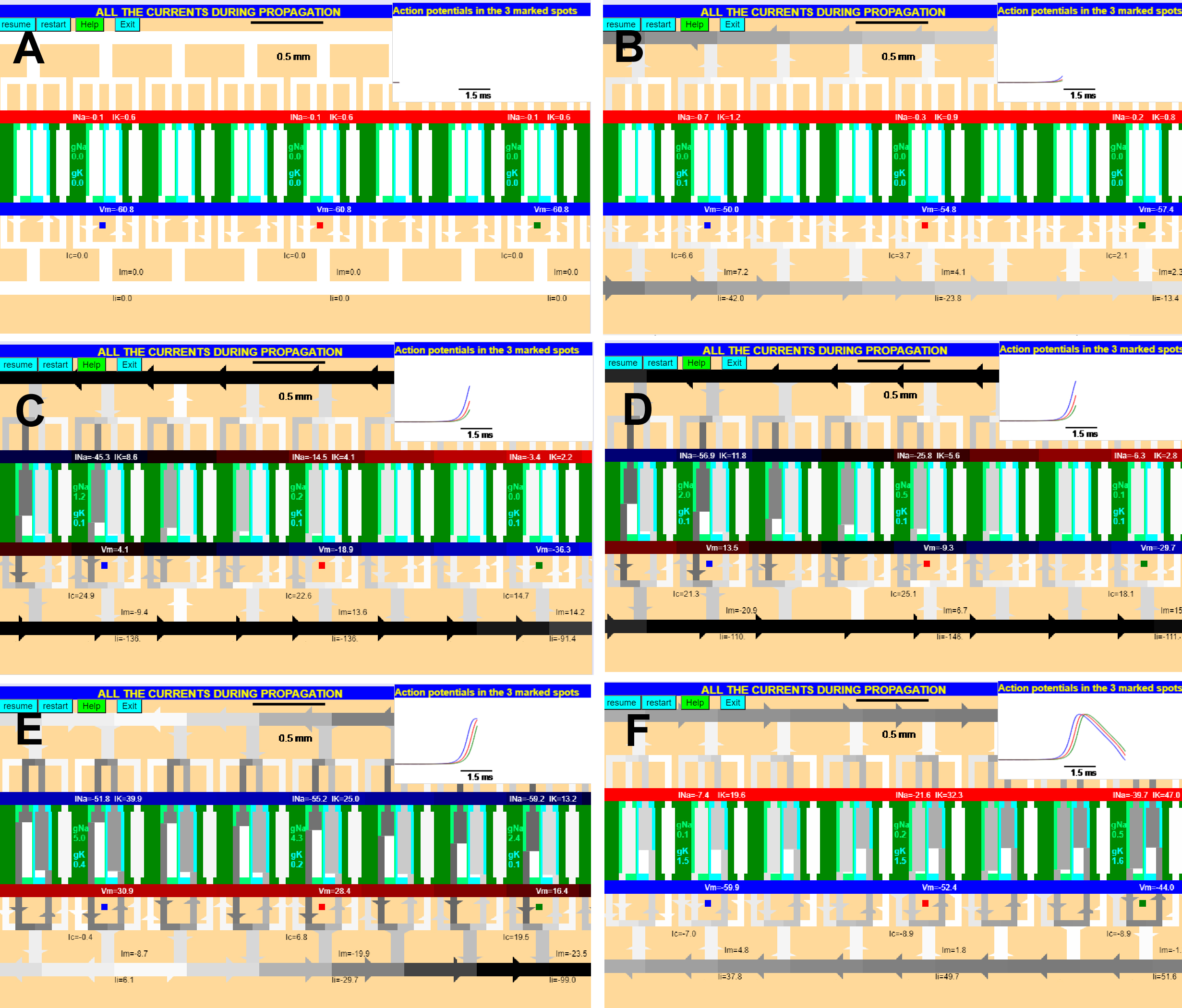
Figure 34. The currents underlying the propagation of the action potential simulated with several consecutive patches. The stimulating electrode is far away to the left of the two pictured patches color-coded red and blue. The time course of the action potential in each patch is shown above each panel and follows the color of the patch. The me Eight membrane patches of a long axon are presented connected between Membrane potential in three of the patches is indicated in internal plate of the capacitor. The currents are shown in each branch and the values of the conductances are shown for the Na conductance (gtreen) and K conductances (cyan) in three of the patches. .
It is important to realize that the described process of current circulation between patches is continuous and not as discrete as it may appear from the figure. In fact the depolarized region is a large stretch of axon that has no exact boundaries. Notice that the action potential reaches its peak in the blue patch before it does in the red patch (Fig 34E) and that the repolarization in the blue patch preceeds the red and green patches (Fig. 34F). This means that there is a propagation time between the patches; therefore in a long axon it will take time for the action potential to propagate from the initiating site. The cable properties are important in determining the propagation of the action potential. We have seen that the space constant, l gives an indication of how far the current passively spreads down along the axon. A long space constant will allow the depolarization of the active patch to reach further than a short space constant. Consequently a long space constant will help in a faster propagation of the action potential. Factors that influence l, such as the internal resistance, membrane resistance or external resistance along the axon will have an influence in the conduction velocity. Remember that the value of l is proportional to the square root of the fiber diameter. If all other factors are maintained constant, such as resistivity, specific membrane conductance and specific capacitance, then we would predict that increasing fiber diameter increases conduction velocity. The giant axon of the squid, which is about 500 mm in diameter, can propagate the action potential at about 18 meter/s, whereas C fibers in vertebrates are around 1 mm in diameter and propagate the action potential at about 1 m/s.
Myelinated Axons
Another strategy for fast propagation is utilized by vertebrates with axons
that are covered with and insulating layer (myelin) that is
interrupted periodically exposing the axon in the nodes of Ranvier . In this case, the circulation of current between patches is indeed discrete
because there is a very good insulator (the myelin) that covers the axon between
nodes of Ranvier. The myelin is formed by a glial cell that envelopes the axon
with multiple turns where each turn is just the membrane of the glia. The result
is that the internal medium is insulated from the external medium with multiple
membranes increasing the membrane resistance (or decreasing membrane
conductance) significantly. At the same time, as each membrane is a capacitor,
the inside is separated from the outside by many capacitors in series,
decreasing the total membrane capacitance significantly. (This is because when n
capacitors, each of value C, are connected in series the total capacitance is
C/n). The very low membrane conductance and very low membrane capacitance in the internodal region is essentially
a passive membrane. The activation of the Na conductance occurs in the nodes
where the action potential develops. An active node of Ranvier will excite its
neighboring node by the same mechanism outlined above, except that because the
nodes are separated by the myelinated region and are so far apart, the actual
speed of propagation is increased even when the fiber diameter is not very large.
For this reason this type propagation has been called saltatory conduction.
You can observe the effect of the myelin in an axon by running the Nerve program
and selecting the propagated action potential mode. Then, go to AXON PROPERTIES
and click on Non-Mielinated (to change to mielinited) and then run the
simulation againin either V vs T or V vs X modes. When using V vs X mode you
will see why is called saltatory.You can also see how the currents spread
between nodes. To start click here.
NOTES:
1. A potential difference exists between two points whenever the introduction of a conducting path between the two points would result in spontaneous charge transfer or electric current.
2. An electric capacitor is a device that allows the separation of electric charge on two conducting plates by a material, or dielectric, that is not able to sustain an electric current.
3. The electromotive force of a battery is the voltage measured from the battery in the absence of current circulation
4. The Hodgkin and Huxley formulation assumes independence between activation and inactivation giving origin to m3h. The predictions of the action potential mechanisms are not modified by using independence or coupling between activation and inactivation.
5. If the capacitor is ideal and there is no resistance in series, the application of a voltage V will produce an infinite amount of current in an infinitesimally short time transporting a charge q=CV. In practice V is not an step and there is a series resistance, therefore the capacitive current will last a finite time.
6. In the axon, part of the membrane capacitance is a function of voltage due to the gating mechanisms but it is a small fraction that has a negligible effect in the interpretation of the action potential generation