INTRODUCTION

The computer experiments described below are designed to explore the properties of excitable membranes and their ability to generate action potentials. These experiments are based upon the squid giant axon, however, the principles that you learn here can be directly applied to action potentials in any other nervous system. The squid giant axon was the biological preparation where all the original experimental information was obtained by Hodgkin and Huxley. These investigators developed a set of differential equations that reproduces the experimental situation accurately. The equations are based on physical principles and they can be solved by digital computers allowing the operator to change parameters and conditions to study the effects on the electrical response of the axon.

While performing these computer experiments, you will be learning how ionic conductances, currents, and membrane voltage are related and this knowledge will provide a strong foundation for understanding heart and synaptic function as well. In each exercise there is a basic experimental setup which gets you going, then you are asked several specific questions. You then perform "experiments" to answer these questions. Be sure to keep track of what you do experimentally, since the results from earlier experiments may help you later in the more complicated experiments.

Current Clamp vs. Voltage Clamp

The axon properties can be studied under two different kinds of stimuli: Voltage clamp or Current clamp. In voltage clamp mode, the experimenter controls the voltage and measures the current and it is the most effective way to describe the properties of voltage dependent channels. Under voltage clamp the membrane potential is constant, therefore there is no capacitive current (except during the instant when the voltage is stepped from one voltage to another)

In this laboratory, most of the experiments are in current clamp mode. The experimenter applies current pulses and observes the voltage response. This is closer to the physiological conditions of axon operation and experiments done under these conditions will give a closer insight as how the normal axon works. This mode is harder to understand because the voltage is controlling the conductances which in turn are allowing ionic currents to go through the membrane which in turn modify the membrane voltage. In addition, as the voltage is changing, there is a capacitive current that is contributing to the total membrane current. It is then suggested that you go through experiments 1 through 6, which are in current clamp mode and, optionally, go to experiment 7 to perform voltage clamp experiments to review your knowledge of how voltage dependent channels operate.

Membrane vs. Propagated action potential.

 As we are dealing with an axon, changes of V in one spot may be different in other regions of the axon. In the Membrane Action Potential window we eliminate this problem by inserting an axial wire and making the membrane isopotential ("space clamp condition"). In the Propagated action potential window, the axon does not contain the axial wire. To simplify the interpretation, all the initial experiments are done with the axial wire.

PROGRAM SETUP

Start the nerve program. If the program was running, some of the parameters may be different from the default values. To correct this, start the program again which will revert all parameters to their default values. The access to the different simulation modes is by way of the buttons on the top of the main screen, as shown in Fig. 1.For example, to initiate an action potential simulation with axial wire, just click on the Membrane AP button. This action will open a window that has a plotting area and several buttons to perform different operations.

EXPERIMENTS

The initial experiments are designed to familiarize you with the different variables that are useful in understanding the generation of the action potential.

Experiment 1:

To start, click on the Membrane AP button. You should see a plot of the voltage as a function of time (black trace) along with the current pulse used to stimulate axon, also as a function of time (red trace, see Fig. 2). What you have done is to simulate with the equations the injection of a current pulse (of 10 mA and 0.25 ms duration) to the axon and record the membrane potential. These are the default values and you will be able to change them in the course of the following experiments.

 So, you have generated an action potential! Now we will ask what is underlying this phenomenon. Let us explore what is the time course of some of the variables that may be changing during the generation of the action potential. The program allows you to plot in he same screen the time course of many of the important variables.

For example, let us look at the potassium current and potassium conductance during the action potential. Click on the VARABLES TO PLOT which will open the Variables to Plot window, and click on the potassium conductance (g_K) and the Potassium current (I_K).

Now you should see plots of the membrane voltage, g_K, and i_K. (Fig. 3).

In which direction is the potassium current flowing, into or out of the cell?

In the VARIABLES TO PLOT window you will find Select scale. Here you can select the scale of  the plotted variable on the right side. . You can also vary the range for the g_K and I_K plot by expanding or  compressing the plotted scales using the Ex and Cc buttons. For example, after you have clicked to display g_K, the default scale will be 20 mS/cm² and if you press Ex, the maximum scale will read 10 mS/cm² and the g_K trace will be twice as big, allowing you to see more details. Press Cc to go back to the original scale. To make comparisons easier between different variables you can select a different plotting scale for I_K. Also, as before, you can display the legend and scale for each variable by selkecting in the lowe panel of the Variables to plot window. In addition, by clicking the mouse in the plotting area, a vertical cursor appears and the values of time, voltage and INa, IK and Ii are printed at the time signaled by the cursor (see Fig. 5 to see how the cursor looks like). Notice that the time courses for i_K and g_K are different. The i_K curve reaches its peak before g_K, why? [Hint: display the equilibrium potentials (by clicking on E's  button) and consider the relationship between E_K and the membrane voltage.] Observe the falling phase of the potassium current. How can the potassium current (I_K) have fallen to nearly its resting level while g_K is still greater than 0? Is I_K equal to 0? You can check this more accurately by using a higher gain (higher magnification using the Ex button) for the I_K plot. Once you understand the reasons for the different time courses of I_K and g_K, add the n curve to your plot. The screen should look like figure 4. The n curve is a measure of the time course of the opening and closing of one of the four subunits of the potassium channel (often referred to as the opening and closing of the n gate). Select the  scale  for the n curve. Remember that the probability of opening P_o=n⁴ and that g_K=NP_o. What is the significance of the fact that the n curve does not start at 0? Why is I_K nearly 0 at the end of the action potential trace even though at this same time n is even greater than its resting value of approximately 0.4?

 After this you may consider how sodium ions are involved in the action potential. Click on Variables To Plot to deselect the potassium variables and check the sodium variables I_Na and g_Na. You should see plots of the membrane voltage, g_Na, and I_Na. Remember, as before, you can display the legend and the plotting scales that are best for comparing g_Na and I_Na selecting the corresponding scale. Figure 5 shows the screen with g_Na, I_Na, and membrane voltage plotted. Notice that the time courses for I_Na and g_Na are different. In which direction is the sodium current flowing during the action potential? There are several interesting and important features shown in the sodium current trace. First, why is there a notch in the I_Na trace? What can you learn from this about the relation between I_Na and g_Na? [Hint: display E_Na and consider the relationship of E_Na to the membrane voltage V.] Notice that the peak I_Na curve occurs later than the peak of the g_Na curve, why?

Once you understand the reasons for the different time courses of I_Na, and g_Na, add the m and h curves to your plot. Note: these variables can best be understood if you simplify your screen by removing the sodium current (deselect I_Na in Var. To Plot). Now you can compare the time course of the membrane voltage and the m and h curves during an action potential along with g_Na (which is proportional to m³h). The screen should look like figure 6. Click on the right hand scale to display the legend for the m or h curves. What is the significance of the fact that the m curve does not start at 0 and that the h curve does not start at 1?. Remember that m represents the probability that one of the subunits is in the active position and in the classical formulation three are required to open the channel (m³) but at the same time, the inactivation particle has to be out of position for the channel to conduct. The probability that the inactivating ball is in position is given by 1-h. Therefore the probability that the Na channel is conducting will be: P=m³h and the conductance will be g_Na= N_NaP = N_Nam³h. Thus, from these two curves you can get an appreciation of how the two gates of the sodium channel can act to regulate the sodium channel's permeability. To see how these interact, plot g_Na, m, and h together. Why does the sodium conductance begin to fall even though the sodium channel's m gate is still open? What would occur if you tried to stimulate the nerve with a second pulse timed to coincide with the peak of the sodium conductance? Don't do this experiment now, just think about it; you have enough information to make a definitive statement. In fact, now you should be able to explain the ionic mechanism responsible for the absolute and refractory periods (more on this later).

   Lastly, examine the total ionic current that flows during an action potential. Deselect the sodium variables and check the total ionic current (I_i) in the Variables to Plot window. This is shown in Figure 7. Note that there are 4 points in time during the trace at which the net ionic current is zero. To really see the four points you must increase the vertical gain of the total ionic current. Click on the right hand side vertical scale until you see Ii and then click on the Ex button several times until you see full detail of the ionic current.

Identify these points and consider their significance.

Remember that this is a membrane action potential, therefore the total membrane current is equal to the sum of the capacitive current plus the total ionic current: I_m=C(dV/dt) +I_i However, after the current pulse is finished, I_m=0 and we have

I_i=-C(dV/dt)

Use this equation to relate the total ionic current to the slope of the membrane potential at different points during the action potential.

Can you explain why the peak inward current occurs before the peak of the membrane voltage? Think back to your study of the sodium conductance. Look at the total ionic current during the falling phase of the action potential waveform and compare to the rate of decay of the action potential.

NOTE: At this point, you may like to review your understanding of the voltage dependent conductances to be able to interpret the previous results and the next experiments. If you feel this is the case, then this is a good time to proceed to experiment 7, before continuing with experiment 2.

Experiment 2:

 This following set of experiments is designed to analyze the properties of membrane action potentials under a variety of different conditions. Start from the membrane action potential window with a simple action potential simulation as in experiment 1. The simple way is to restart the program and click on the membrane action potential. Set up the stimulus parameters(click on PULSES) for a single 0.25 millisecond duration pulse with a 10 microamp amplitude. . Run this action potential simulation. This should produce a fairly broad time course for the action potential. Notice that the action potential actually begins after the stimulus pulse is turned off. How is this possible? It will help to plot the total membrane current and the Na and K currents in a magnified vertical scale. After you have understood why the action potential starts after the pulse, remove the extra variables (if you added them) by deselecting them in the Var to Plot window.

Before increasing the temperature, press SUPERIMPOSE which will allow you to superimpose the traces at two different temperatures. So far you have been working at the default temperature of 6.3^o C, now, increase the temperature to give a faster action potential waveform. To do this, click on AXON PARAMETERS and window will appear. The temperature can be changed by typing a value in the window followed by the ENTER key. You will notice that as the temperature is varied, the action potential generated has different shape and it will show superimposed on the 6.3 C action potential and an example is shown in Figure 8.

Try several different temperatures. What happens to the action potential as the temperature is increased? Since the reduction in action potential amplitude cannot be accounted for by changes in E_Na or E_K, what then accounts for these changes? [Hint: consider the effect of temperature on channel kinetics] Why does the action potential start sooner as the temperature is increased?

Experiment 3:

Based upon Hodgkin and Huxley's formulation, the action potential should be made up of an inward sodium current and outward potassium current. If this is so, then when the external ion concentrations are changed the action potential waveform should change in predictable ways. We can test this directly by first changing the external sodium concentration. Reset everything by restarting the program and clicking on Membrane action potential. Since we will be examining the effects of decreasing the external sodium concentration we need to increase the stimulus to insure that an action potential will occur each time. Click on Pulses and set the stimulus strength to 20 microamps and increase the total time to 12 ms.

To simplify interpretation we will first run this simulation using ideal Na and K channel properties where only sodium or potassium ions go through their respective channels (ie in an ideal Na channel only Na can permeate). Then we will return to more realistic channel properties (Hodgkin and Huxley type Na and K Channel properties) where both ions can pass through each channel with preferential permeability ratios (for example a real, or HH, Na channel conducts Na 15 times better than K). To do this, in the Axon Parameters window click on the ideal Channel Properties.  Click now on SUPERPOSITION and then click on CONCENTRATIONS and modify the external sodium concentration from its default value which is 440 mM to 200 mM. You will see now the new action potential superimposed in the reference Action potential recorded in the default external Na concentration. Progressively reduce the external sodium concentration and observe the action potential. Before you run these simulations with reduced sodium concentrations try to predict what changes you will see. If you do not wish to superimpose clkick on NO SUPERIMPOSE. When you have reduced the external sodium concentration to about 200 mM, the superposition should look like the action potentials shown in Figure 9. Notice that there is a small change in the resting potential. Why does this occur if the resting potential is mainly determined by the potassium concentration? Also note that many aspects of the action potential waveform have changed (e.g., rate of rise, peak amplitude, and the overshoot) but the undershoot did not. Be sure you can explain each of these changes in terms of the changes of the external Na concentration and E_Na (Click on E's to display the equilibrium potentials). In this experiment the effects and interpretation of the sodium concentration changes were simplified by using idealized channel properties.

Optional: For a more realistic view of the effect of sodium, repeat this experiment using normal non-ideal channel properties (In the Axon Parameters window, check the non-ideal Channel). Again, try to predict the effect of the sodium concentration changes. Figure 10 shows two superimposed action potentials recorded in 100% and 40% of normal sodium concentration outside. Examine the effects of the 40% sodium concentration on the action potential waveform. Explain why the changes in the action potential waveform are different when normal rather than ideal channel properties are in use. What happened to the resting potential and the action potential undershoot, why? How do these changes compare to those seen using ideal sodium channels? Be sure that you understand and can explain these differences.

Experiment 4:

In experiment 3 we saw that changes in external sodium affected many of the action potential properties. Let us now examine the threshold, which is a property that defines whether the action potential will or will not be generated. Restore the action potential parameters by restarting the program. In the Pulses window change the amplitude to 10 uA and the total duration to 10 ms. Now, experimentally determine the amplitude of the current pulse that is required to just exceed threshold (that is, that generates an action potential). To see the relationship between different stimulus intensities you can click superimpose so the traces will superimpose as you change the stimulus strength.  Figure 11 shows one example of a series of superimposed traces, the suprathreshold stimulus was 5 uA and initiated an action potential but a 4.8 uA did not.

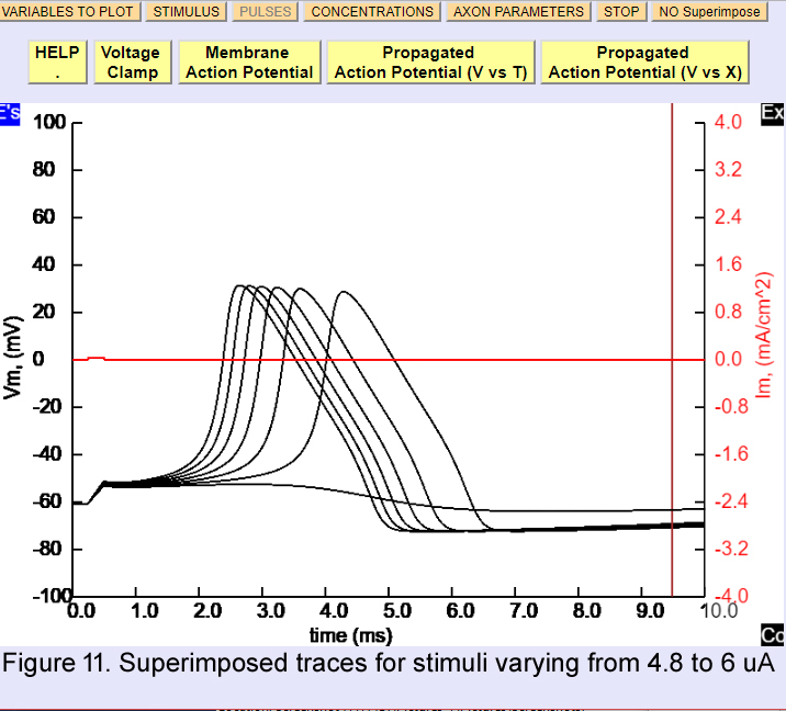Experiment with the amplitude and observe how sharp is the threshold. Why does the progressive reduction of the stimulus intensity cause the onset of the action potential to occur at progressively longer times after the cessation of the stimulus? [Hint: One suggestion as to how to approach answering this question is to try examining the total ionic current at high magnification, together with the Na and K currents. Observe the direction of the currents just when the action potential is taking off]. Also, why when the stimulus is just at threshold, does the membrane potential remain depolarized past the turn off of the current pulse? Try now to correlate the threshold events with the conductances (and also plot the h variable). Once you see how the membrane voltage is related to the membrane conductances you should be able to explain why the stimulus that is just suprathreshold generates a smaller than normal action potential (i.e., compared with the action potential resulting from a stimulus of 10 microamps).

Note the value of E_K and membrane potential V. Now increase the extracellular potassium progressively and examine its effect on the action potential and threshold. Be sure to examine g_K, g_Na, m, n, and h. Try 20 mM extracellular K. Why do comparatively small changes in potassium have such a profound effect compared to the effect of sodium concentration changes that you tried in experiment 3? Furthermore, why do large changes in potassium actually stop all activity? Examine the changes in membrane potential, the m,n and h variables and the equilibrium potentials.

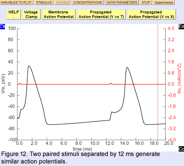
Experiment 5:

So far we have been examining the properties of a single action potential, but now we will study how one action potential can affect the generation of a second action potential. First restore default parameters by restarting the program and then in the pulses window increase the total time to 20 ms and add a second pulse (increase pulse 3 to 10 microamps Amplitude, and 0.25 msec Duration. Then modify the duration of the second pulse (which is an interval with no pulse) to 12 msec. Make sure that the first and the third pulses are the same. You should see two action potentials as shown in figure 12.

 Now we will change the first stimulus, PULSE 1, and see how this affects the second action potential. Press Superimpose. First, progressively decrease the amplitude of PULSE 1 and observe the second action potential waveform. When you decrease PULSE 1 to an amplitude that is very near to threshold (i.e., S₁ set between 6-7 microamp), the second action potential is abolished (Figure 13;here PULSE 1=6 microamp). Try different amplitudes for PULSE 1. Why does PULSE 3, which was previously suprathreshold, now become so much less effective in eliciting an action potential and even become subthreshold if PULSE 1 is made small enough? How can you change PULSE 3 to elicit the second action potential?

Now let us explore the generation of a second action potential as a function of the separation of the two stimulii. In the Stimulus window reset the first stimulus to 10 microamp and 0.25 ms and change the Interval to 6 ms. Keep changing the stimulus amplitude of the second pulse until you have a nice action potential. Then repeat this process by making the interval even shorter and modifying the amplitude of the second pulse to recover the second action potential. Why you cannot obtain a second action potential regardless of the amplitude of the second pulse when you decrease the interval below a critical level?. What do these results tell you about refractory periods and threshold? Be sure that you understand the mechanisms underlying these processes. Try to explain these results remembering what you know about Na inactivation and potassium activation. A simultaneous plot of h and g_K are very useful.

There are many physiological factors that can affect the excitability of a cell. Dramatic changes in excitability can occur, for example, in response to small changes ionic concentrations or when cells are exposed to very small concentrations of drugs and toxins. You may want to study some of these effects on your own using this program.

Experiment 6:

Restart the program. Then click on the  Propagated AP (V vs T) and observe the normally propagated action potential at three points along the axon. Compute the conduction velocity. This can be easily accomplished using the cursor feature. Click with the mouse at the peak of the blue action potential and you get the time and the value of the voltage at the three recording electrodes: take note of the time (see Figure 14). Next, click on the the peak of the red action potential and take note of the time. Knowing the time difference and the distance between the electrodes you can compute the conduction velocity. Next, test whether the conduction velocity is temperature sensitive by rerunning the simulation at different temperatures. Examine the kinetics of m, n and h.

How do you account for the changes in the action potential's shape (waveform) and size at higher temperatures? Now set the temperature to 18^o C and change the diameter of the axon to 400 microns.What happened and why? You should know a variety of different ways to alter this experimental situation to cause an action potential in this new cell. First try to increase the stimulus intensity. Calculate the new conduction velocity for this larger diameter cell. Run the simulation using a 100 micron diameter axon. Before you run this simulation consider the magnitude of the stimulus pulse. What type of a voltage response do you expect in the nerve if you use the same stimulus parameters as you used with the 400 micron fiber? After you adjust the stimulus intensity to fire an action potential in the 100 micron fiber calculate the conduction velocity. What is the effect of fiber diameter on conduction velocity? Be sure that you can give an explanation of the mechanisms responsible for these changes in conduction velocity.

 Cable properties of the axon. Now that you have seen the propagation due to the presence of the voltage dependent conductances it is a good moment to see what happens without them. Prepare the program as follows. First, click on the Axon button (or press F6) and reduce the maximum sodium and potassium conductances to zero. Then click on the Pulses button and adjust the total time to 20 ms and the amplitude of PULSE 1 to 5 microamps and the duration to 12 ms.  With the mouse, drag the center electrode closer to the stimulus, say to to 0.5 cm. Wait for the next try toi see the correct response after the change in parameters. You see now the passive response of the axon to the stimulus at the stimulating site but there is almost nothing that you can detect with the third electrode (Figure 15)

.

Now you see the response, slowed down and attenuated at the blue electrode position. Keep changing the electrode position and so you can have an idea of how fast the passive response is attenuated along the axon. Use the cursor and then try to estimate from these measurements the value of the space constant.

Finally,run the Voltage versus distance by clicking on the VvsX propagated AP and verify the extent of axon that is depolarized during an action potential. Notice that the depolarized region is a relatively long stretch of axon.

Experiment 7 (optional):

This experiment will be done under voltage clamp. Restart the program and click the Voltage clamp button. This will present a simulation of a voltage pulse from -70 to 0 mV for 10 ms (black trace) showing the ionic current (red trace) with its inward Na component and outward K component. (Figure 16). To see the Na and K components, click on Variables to Plot and add I_Na and I_K Click on the right hand scale until I_Na is displayed and then click on the Cc button to compress the current so it will have the same scale as I_m. Repeat the same operation with I_K .

 Deselect I_Na and I_K and proceed now to give a family of voltage clamp pulses restart the problem and cklick on voltage clamp. Decrease the maximum scalec pressing Cc twice. In the Pulses window change the amplitude to -60 mV, then check Family and modify the pulse Pulse 2 (from) to -60 and the Pulse 2 (to) to 60 mV. If you press Superimpoose, all the traces will look like in Fig. 17

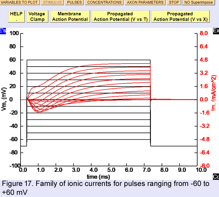
Identify the Na and K current components and notice when the Na current turns outward. Click on CONCENTRATIONS and add Tetrodotoxin (TTX). The simulation will run on top of the previous family. To clear the old family, click onno superimpose. Now you can see the K currents in almost isolation. Identify the turn on time, lag and maximum current for each potential.

Study the gating of the sodium current. Decrease TTX to zero. Uncheck family and change the pulse amplitude to -10 mV. In Var To Plot select I_Na, m and h. Go to the Physiological parameters menu and increase TTX to the maximum.

Further experiments suggested are: 1. settling of inactivation using a double pulse protocol where the amplitude of the pulse 2 is varied and pulse 3 is fixed; 2. recovery from inactivation, where pulse 1 is fixed at 0 mV for a duration of 10 ms, pulse 2 at -70 (or other potential) with a variable duration and pulse 3 is fixed at 0 mV with 2 ms duration.